
FD-Align: Feature Discrimination Alignment for Fine-tuning Pre-Trained Models in Few-Shot Learning
Background
CLIP demonstrates exceptional performance across various visual tasks. When applying it to downstream tasks, it often requires fine-tuning on the downstream data. However, in few-shot learning, directly fine-tuning CLIP can easily lead to overfitting and adversely affect its generalization on out-of-distribution (OOD) data. Consequently, previous methods have mostly attempted to fine-tune only the classification head or introduce additional structures, but these approaches do not fully exploit the potential of CLIP’s visual encoder. Therefore, our research explores how to fine-tune CLIP with a sample number of samples without decreasing its performance on OOD data.
Motivation
We explain the decline in OOD performance of fully fine-tuned CLIP through the robustness to spurious correlations. This robustness refers to the model's ability to distinguish between causally relevant information (related to the class) and irrelevant information (such as background or style), which are spurious. Previous work has shown that CLIP exhibits strong robustness against spurious correlations, thus ensuring impressive OOD performance [1]. However, fully fine-tuning of CLIP results in a decrease in its OOD performance [2]. Visualizing the attention maps of both CLIP and its fully fine-tuned counterpart reveals that the fully fine-tuned CLIP tends to focus more on localized features. This heightened attention to local areas weakens the model's robustness against spurious correlations [3]. In other words, while fully fine-tuning enables the model to better learn the causal features of the fine-tuning samples, it diminishes its capacity to recognize spurious correlations, which leads to the casual features extracted by the model failing to generalize to unseen samples, resulting in overfitting and impaired generalization on OOD data. Therefore, we proposes a fine-tuning methodology that does not compromise the model's ability to recognize spurious correlations, thereby preserving the robustness of the fine-tuned model against spurious correlations.
Method
We aim to fine-tune CLIP’s visual encoder $f_0$ on a few-shot dataset $\mathcal{D}\subset\mathcal{X}\times\mathcal{Y}$ to obtain $f_t$. Our approach is divided into two parts: model fine-tuning and spurious feature constraint.
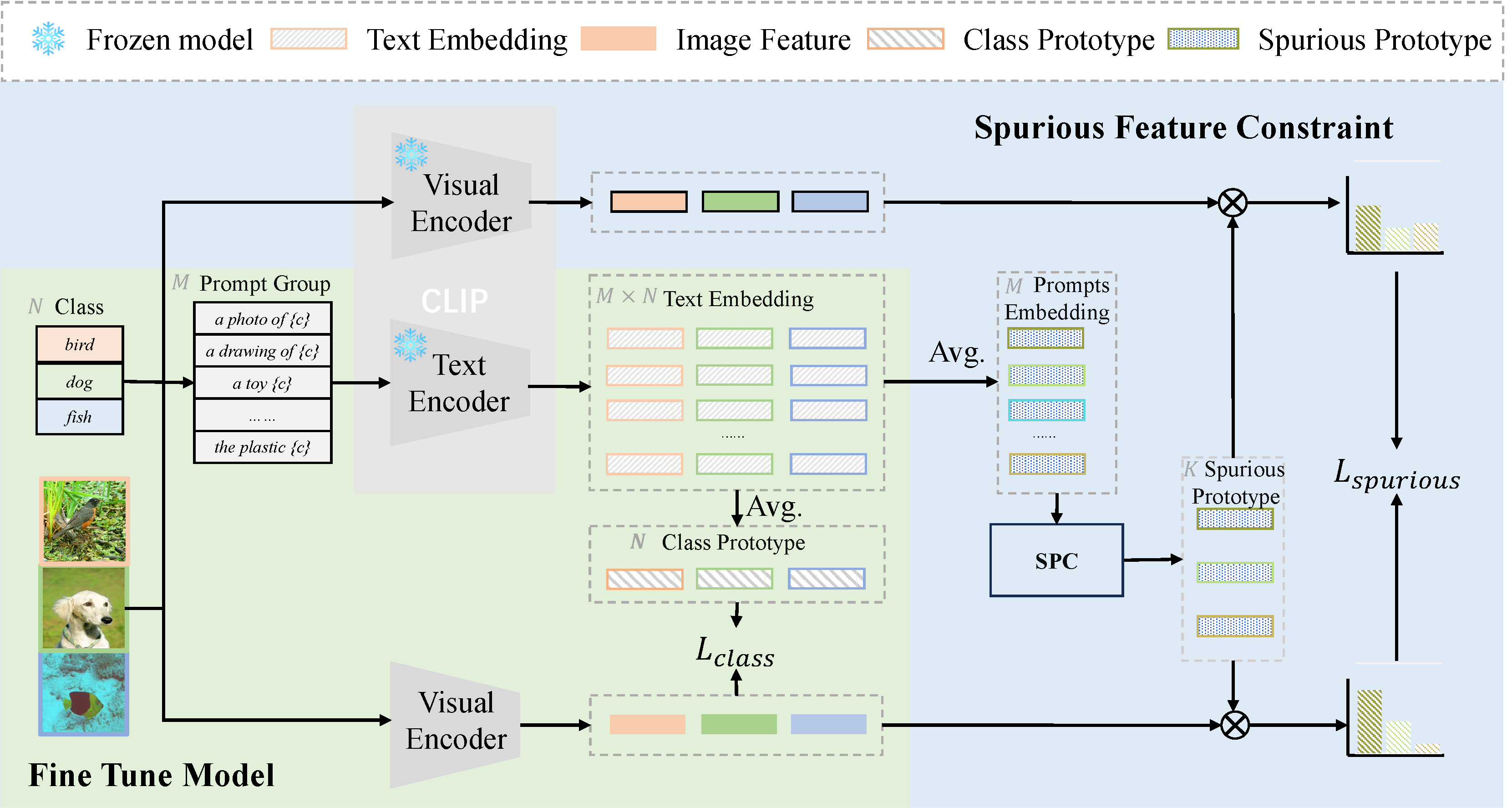
Model fine-tuning
During the fine-tuning process, CLIP's text encoder $g_0$ is frozen. We input images $x$ along with their corresponding label $y$ and $M$ prompt templates $(P_1, \cdots, P_M)$. For any given category $y$, its associated prompts are denoted as $[P_1, y], \cdots, [P_M,y]$. For each category $y$, we utilize the text encoder to extract features from all prompts, which are then used to compute the prototype of that category.
\[\mu^{\text{class}}_y:=\frac{1}{M}\sum_{j=1}^M g_0([P_j, y]). \nonumber\]We calculate the similarity between the image and the category prototypes using cosine similarity, and then compute the probability density accordingly. Subsequently, we employ cross-entropy loss as the classification loss during the fine-tuning process
\[\mathcal{L}_{\text{class}}=-\frac{1}{|\mathcal{D}|}\sum_{(x_i,y_i)\in \mathcal{D}}\log\frac{\exp(s(f_t(x_i), \mu^{\text{class}}_{y_i}))}{\sum_{y\in\mathcal{Y}} \exp(s(f_t(x_i), \mu^{\text{class}}_y))}, \nonumber\]Where $\mathcal{Y}$ is the set of label.
Spurious Feature Constraint
Ensuring the constancy of spurious features during fine-tuning is most directly achieved by decoupling causal and spurious features, while maintaining the stability of the spurious features. However, decoupling features in images is an extremely challenging task. In contrast, it is much simpler to decouple spurious and causal features in text. For example, in the prompt 'a photo of a dog,' 'dog' is the causal feature, whereas 'a photo of a' represents spurious features. Leveraging CLIP's strong alignment capabilities between vision and text, we can use the spurious features in text as prototypes for the spurious information in images
\[\mu^{\text{spurious}}_{P_j}:=\frac{1}{|\mathcal{Y}|}\sum_{y\in\mathcal{Y}} g_0([P_j, y]).\nonumber\]We can obtain the probability distribution of image features extracted by the fine-tuned model on spurious information:
\[\mathcal{P}_{\text{spurious}}(x; f_t)=\operatorname{SoftMax}\left[s\left(f_t(x),\mu^{\text{spurious}}_{P_1}\right), \dots, s\left(f_t(x),\mu^{\text{spurious}}_{P_M}\right)\right].\nonumber\]Meanwhile, We can obtain the probability distribution of image feature extracted by CLIP on spurious information:
\[\mathcal{P}_{\text{spurious}}(x; f_0)=\operatorname{SoftMax}\left[s\left(f_0(x),\mu^{\text{spurious}}_{P_1}\right), \dots, s\left(f_0(x),\mu^{\text{spurious}}_{P_M}\right)\right].\nonumber\]Although it is not feasible to directly ensure that the spurious features in the image features extracted by the fine-tuned model and the original CLIP are identical, we can indirectly ensure consistency of the extracted spurious features by constraining their probability distributions on spurious information to be the same.
\[\mathcal{L}_{\text{spurious}}=\frac{1}{|\mathcal{D}|}\sum_{(x_i,y_i)\in \mathcal{D}}\operatorname{KL}\left(\mathcal{P}_{\text{spurious}}(x_i; f_t) \mid\mid \mathcal{P}_{\text{spurious}}(x_i; f_0)\right).\nonumber\]Finally, we constrain both the classification loss and the spurious consistency loss to ensure the OOD generalization of the model during fine-tuning.
\[\mathcal{L}_{\text{total}} = \alpha\cdot \mathcal{L}_{\text{class}} + \beta\cdot \mathcal{L}_{\text{spurious}}.\nonumber\]Spurious Prototype Correction
Currently, most prompt templates are either manually designed or generated by language models, which can lead to unreasonable or redundant scenarios, resulting in inaccurate prototypes of spurious information. To address this issue, we initially employ anomaly detection algorithms to remove unreasonable prompt features.
\[\mu^{\text{spurious}} :={IsolationForest}(\mu^{\text{spurious}}, n).\nonumber\]Subsequently, we utilize the $k-Means$ clustering algorithm to deal with the redundant features in the prompts.
\[\tilde{\mu}^\text{spurious} := \operatorname{k-Means}(\mu^{\text{spurious}}, k). \nonumber\]Experiment
Results on OOD
As shwon in the table below, we conducted 16-shot fine-tuning of CLIP on ImageNet and evaluated its performance on two variant datasets of ImageNet. Compared to fully fine-tuning, FD-Align achieves a comprehensive improvement in OOD performance. Additionally, by directly applying the fine-tuned visual encoder to Tip and APE, it is evident that our fine-tuned model can be applied to existing methods without the need for re-tuning, thereby enhancing OOD performance.
| Method | CLIP | Baselines | Baselines + FD-Align | ||||||||
|---|---|---|---|---|---|---|---|---|---|---|---|
| FT | Tip | Tip-F | APE | APE-T | FT | Tip | Tip-F | APE | APE-T | ||
| ImageNet | 63.34 | 64.91 | 65.49 | 68.43 | 66.55 | 68.74 | 66.39 | 65.49 | 68.70 | 67.59 | 69.15 |
| ImageNetS | 42.31 | 42.24 | 42.48 | 42.54 | 43.28 | 43.23 | 43.50 | 43.84 | 43.67 | 44.23 | 44.04 |
| ImageNetV2 | 55.92 | 57.63 | 57.58 | 59.58 | 58.31 | 59.58 | 57.73 | 59.10 | 60.17 | 59.36 | 60.83 |
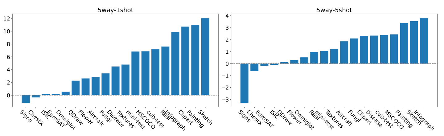
Similarly, we fine-tuned CLIP on miniImageNet following the $N$-way $K$-shot few-shot learning, and evaluated its performance on various downstream datasets. The following figure illustrates the performance changes of the fine-tuned model across different datasets. FD-Align brings significant improvements in OOD performance on most of the datasets.
Results on ID
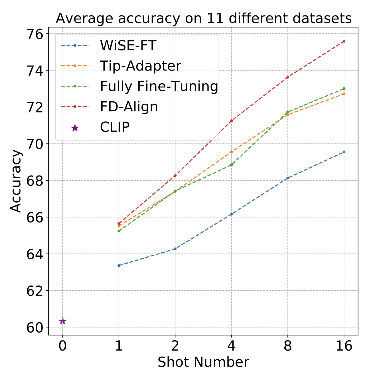
We also evaluated the in-distribution (ID) performance of our method across 11 datasets. Our approach demonstrates a significant improvement in performance, which becomes even more pronounced as the number of shots increases.
Similarly, we applied the fine-tuned visual encoder directly to existing methods. The table below shows the performance on ImageNet. It is evident that our fine-tuned model can also directly enhance the ID performance of existing methods.
| Methods | 1shot | 2shot | 4shot | 8shot | 16shot |
|---|---|---|---|---|---|
| Tip | 64.11 | 64.36 | 64.63 | 65.17 | 65.49 |
| Tip + FD-Align | 64.51 | 65.33 | 65.76 | 66.79 | 67.28 |
| Tip-F | 64.64 | 65.18 | 65.78 | 67.21 | 68.43 |
| Tip-F + FD-Align | 64.86 | 65.61 | 66.11 | 67.58 | 68.70 |
| APE | 65.36 | 65.69 | 66.00 | 66.55 | 66.55 |
| APE + FD-Align | 66.71 | 67.29 | 67.40 | 67.76 | 67.69 |
| APE-T | 65.89 | 66.18 | 66.82 | 67.99 | 68.74 |
| APE-T + FD-Align | 66.84 | 67.37 | 67.81 | 68.73 | 69.15 |
The Necessity of Correcting Spurious Prototypes
As shown in the table below, we compare the ID performance using all prompt features as spurious prototypes, prompt features manually filtered by Tip as spurious prototypes, and spurious prototypes corrected using Spurious Prototype Correction (SPC). As illustrated, prototypes corrected with SPC achieve higher performance compared to using all prompts. Notably, the performance significantly drops when using prototypes from manually filtered prompts by Tip. We attribute this to the retention of the template ‘itap of a {class}’ in Tip, which is removed as an outlier in SPC. Therefore, SPC module can avoid the irrationality of manual filtering.
| Methods | 1shot | 2shot | 4shot | 8shot | 16shot |
|---|---|---|---|---|---|
| CLIP | 60.33 | ||||
| Fully Fine-tuning CLIP | 63.48 | 64.87 | 68.10 | 71.14 | 73.43 |
| FD-Align (80 templates) | 63.90 | 65.64 | 68.10 | 71.30 | 74.03 |
| FD-Align (Tip templates) | 61.14 | 62.39 | 63.37 | 60.34 | 66.30 |
| FD-Align + SPC | 63.92 | 65.68 | 68.63 | 71.66 | 74.38 |
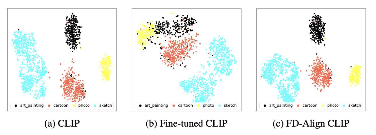
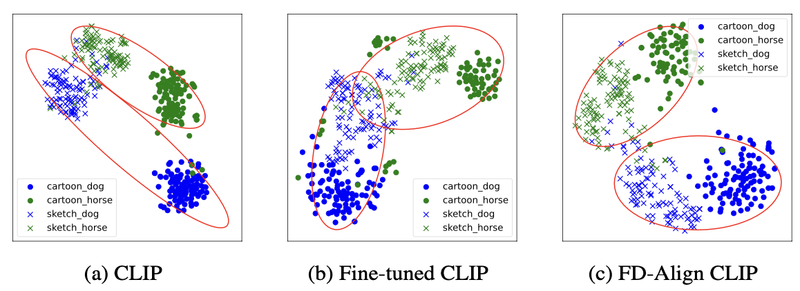
Visualization
We also visualized the image features extracted by different models. FD-Align can distinguish different classes and domains better.
Reference
[1] Self-supervision on images and text reduces reliance on visual shortcut features.
[2] Fine-tuning can distort pretrained features and underperform out-of-distribution.
[3] Are vision transformers robust to spurious correlations?